Run Your First Simulation¶

Use the SDK to create a new project, upload a mesh, run a simulation, and analyze the results using the NACA 0012 Airfoil.

Throughout this page, commands starting with $ should be run in your shell. All other commands should be run in the Python REPL.

The Python REPL can be accessed by running the python command in your shell, without any arguments:

macOS/Linux

$ python

Windows

$ py

Once you’re in the REPL, you can directly execute Python code:

>>> print("hello world")
hello world

Alternatively, instead of running each Python command in the REPL, you can also copy the Python code blocks in this tutorial into a tutorial.py file and run it all at once:

macOS/Linux

python tutorial.py

Windows

py .\tutorial.py

Prerequisites¶

Download the following files:

You will also need the pandas and matplotlib Python libraries to store and visualize the results of our simulation. Install these packages with:

# make sure to activate your virtualenv first, if using one
$ python -m pip install pandas matplotlib

Important

If you’ve never logged in to Luminary Cloud, in your browser, please log in and accept the terms and conditions before proceeding.

Creating a Project¶

We’ll start by entering the Python REPL, where we’ll run all of our commands throughout this tutorial.

Enter the Python REPL:

$ python

Import the luminarycloud package:

import luminarycloud as lc

Important

By default, the SDK connects to the Luminary Cloud Standard Environment. If you are an ITAR customer, you must call lc.use_itar_environment() to configure the SDK to use the Luminary Cloud ITAR Environment.

This call should be made directly after importing the luminarycloud library and only needs to be called once, at the start of your script.

Create a new project called “NACA 0012” with a description:

project = lc.create_project("NACA 0012", "My first SDK project.")

Note

If this is your first time using the SDK, or if it has been 30 days since you last logged in, your browser will open and prompt you to log in to Luminary Cloud. If your browser doesn’t open automatically, the link will be printed in your terminal. Open it and log in as normal.

Check that the project was created:

print(project)

Upload a Mesh¶

Now that we have a project, it’s time to upload the mesh file we downloaded from the prerequisites section of this tutorial. The full list of supported mesh file formats can be found here.

Run the following code, making sure to replace the path with the location of the downloaded mesh file:

mesh = project.upload_mesh("path/to/airfoil.lcmesh")
mesh.wait() # wait for mesh upload and processing to complete

When the mesh is done uploading, mesh.wait() will return the current status.

Obtain the mesh metadata¶

After the mesh is uploaded, it is possible to obtain the IDs associated to the different mesh surfaces. These IDs are used when setting up simulations in order to associate entities such as boundary conditions to the mesh surfaces. In order to obtain the mesh metadata, run the following code

mesh_metadata = lc.get_mesh_metadata(mesh.id)

The mesh_metadata object will include all the surfaces of each volume as well as the names of these volumes.

Run a Simulation¶

To run a simulation, you need to specify the simulation settings. The example settings file you downloaded earlier in the prerequisites section contains a full set of configuration parameters that you can use to run this simulation.

Run the following commands, making sure to replace the path with the location of the downloaded settings file:

sim_template = project.create_simulation_template("API simulation params", "path/to/api_simulation_params.json")
simulation = project.create_simulation(
    mesh.id,
    "My first simulation (via the Python SDK)",
    sim_template.id,
)

The simulation should take a couple of minutes. The following line will wait for the simulation to complete:

print("Simulation finished with status:", simulation.wait().name)

You should see the following message:

Simulation finished with status: COMPLETED

Analyze the Results¶

We will use pandas to store and visualize the results. Run the following command to import pandas:

import pandas as pd

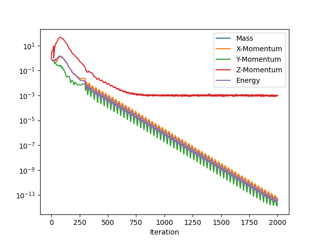
Global Residuals¶

We can start by downloading the global residuals. The function download_global_residuals() returns a file-like object with a read() method. The contents are in CSV format:

# see API reference documentation for more details about optional parameters

with simulation.download_global_residuals() as stream:
  residuals_df = pd.read_csv(stream, index_col="Iteration index")
  # since this is a steady state simulation, we can drop these columns
  residuals_df = residuals_df.drop(["Time step", "Physical time"], axis=1)

print(residuals_df)

Now let’s generate a residuals plot similar to the one found in the UI and save it to a PNG file:

residuals_df.plot(logy=True, figsize=(12, 8)).get_figure().savefig("./residuals.png")

The plot should look like this:

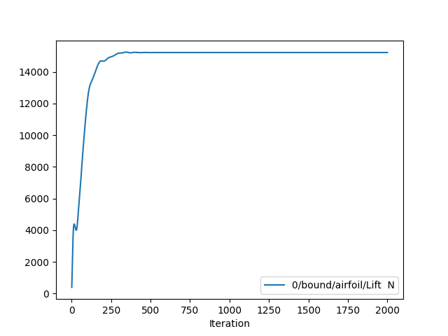
Output Quantities¶

We can inspect output quantities (such as lift) by specifying the quantity type and which surfaces we would like those quantities for.

from luminarycloud.enum import QuantityType, ReferenceValuesType
from luminarycloud.reference_values import ReferenceValues

ref_vals = ReferenceValues(
    reference_value_type = ReferenceValuesType.PRESCRIBE_VALUES,
    area_ref = 1.0,
    length_ref = 1.0,
    p_ref = 101325.0,
    t_ref = 273.15,
    v_ref = 265.05709547039106
)

# see documentation for more details about optional parameters
with simulation.download_surface_output(
    QuantityType.LIFT,
    ["0/bound/airfoil"],
    frame_id="body_frame_id",
    reference_values=ref_vals
) as stream:
    lift_df = pd.read_csv(stream, index_col="Iteration index")
    # since this is a steady state simulation, we can drop these columns
    lift_df = lift_df.drop(["Time step", "Physical time"], axis=1)

print(lift_df)

Similar to before, we can generate a plot and save it to an image file:

lift_df.plot(figsize=(12, 8)).get_figure().savefig("./lift.png")

The saved lift plot will look like this:

Cleanup¶

To exit the Python REPL, use Control-d.

If you were using a virtualenv for the tutorial, you can exit by running:

$ deactivate